Implementing PCA using OpenCV

Here is the implementation of PCA (Principal Component Analysis) using OpenCV 2.4.11.

int DIMENSION;
int DATANUM;
int EIGENNUM;
cv::Mat data;
cv::Mat mean;
cv::PCA pca;

DIMENSION = /* dimension of each datum */;
DATANUM = /* number of data */;
EIGENNUM = DATANUM < DIMENSION ? DATANUM : DIMENSION;

data.create(DATANUM, DIMENSION, CV_64F);
for(int n = 0; n < DATANUM; n++) {
for(int d = 0; d < DIMENSION; d++) {
data.at<double>(n, d) = /* value of n-th data d-th dimension */;
}
}

mean = cv::Mat::zeros(1, DIMENSION, CV_64F);
pca(data, mean, CV_PCA_DATA_AS_ROW, EIGENNUM); // number of eigenvalues and bases is EIGENNUM

// pca.eigenvectors.at<double>(n, d) gives you the value of n-th basis d-th dimension
// pca.eigenvalues.at<double>(n) gives you n-th eigenvalue

In the above example, the mean is not subtracted when calculating PCA.

Implementing PCA

From now on, I explain the detail of implementation. As for the people who cannot understand PCA, the reason is not the implementation detail but the actual data: What kind of output data is obtained depending on input data, what is the meaning of the outputdata. Therefore, I explain the actual example using a synthesized data.

Here is an example of PCA where the average value is not subtracted. This situation is common in computer vision field. Reasons vary widely, and some of them are strong reasons, and some of them are weak reasons. You should think adequately depending on the problem you tackling with. One reason might be to avoid negative value which appears when the mean is subtracted since the image brightness is always non-negative. If the data have offset scaled with a scaling factor which depends on each datum, the offset cannot be represented by the mean but be represented by the basis. Usually, the first basis can be used as offset, and the basis resembles the average data. Therefore, the average value is not needed to calculate because the first basis is similar to the average value. If the mean is subtracted, the paper's formulae might be complex, or the program's code might be complex. The outlier is also averaged, and the mean is contaminated by the outlier. The first basis is deformed by outlier, but the outlier slightly dissappears.

In the computer vision field, data number is often less than dimension number. Pattern recognitions use larger number of data than dimension, but photometric methods use smaller number of data than dimension. For example, photometric linearization, suppose that we took 100 images of 1M pixels. One data is made by arranging the pixel brightness vertically extracted from one image. Therefore, the dimension number is 1M and the data number is 100. This is one example, but there is many examples when the data number is less than dimension number.

If the eigenvalue is close to zero, SVD is stable than PCA. This page skips to explain SVD. Please study by yourself for SVD.

Calculation like PCA need the precision of 64bit floating number (denoted as "double" in this webpage), not the precision of 32bit floating number (denoted as "float" in this webpage). However, for file output, double precision is not needed, float precision is enough, and float array is used for memory efficiency. Therefore, use float for data memory, and use double for calculation. No, be careful! There are some numerical library which calculates using float values if the float values are input. As a result, use double for data memory. Memory might be large, so compile in 64bit not 32bit.

The following example is for Windows 8.1 64bit, Visual Studio Community 2015's Visual C++, OpenCV 2.4.11. Other cases are left for your homework.

OpenCV and Visual Studio

Install OpenCV. Explanation for install is skipped.

Add "C:\OpenCV2.4.11\build\x64\vc12\bin" and "C:\OpenCV2.4.11\build\x86\vc12\bin" to PATH, and reboot Windows. Choose x64, not x86, for Visual Studio's platform. Add "C:\OpenCV2.4.11\build\include" to additional include directory. Add "C:\OpenCV2.4.11\build\x86\vc12\lib" or "C:\OpenCV2.4.11\build\x64\vc12\lib" to additional library directory (Now, I am talking about x64, so latter is added). Adequately modify these directories depending on your install enviroment.

Add below to your source code.

#if _DEBUG
#pragma comment(lib, "opencv_core2411d.lib")
#pragma comment(lib, "opencv_highgui2411d.lib")
#pragma comment(lib, "opencv_imgproc2411d.lib")
#else
#pragma comment(lib, "opencv_core2411.lib")
#pragma comment(lib, "opencv_highgui2411.lib")
#pragma comment(lib, "opencv_imgproc2411.lib")
#endif

#include <opencv2/opencv.hpp>

File format

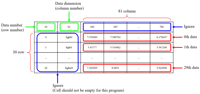
Here, input file and output file are CSV file with comma-separated. Sample program here uses strtok function for reading file. strtok function skips empty items in CSV file. Fill all elements (cells) with a certain values or strings. If you have time, I recommend you to modify the program without using strtok function.

Number of data is written in 0th row 0th colum, and dimension of data is written in 0th row 1st column. 1st and following rows are the data. Ignore 0th and 1st columns, and the data is in the 2nd and following columns. In this webpage, the number starts from 0, not 1. I know that expression such as 0th is unnatural in numbering, but I use this expression so that the students who actually implement this software.

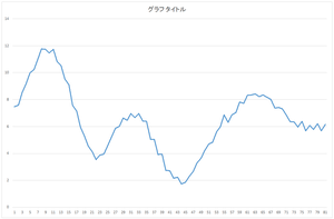
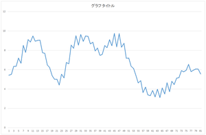
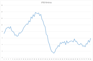
I explain using this file. Number of data is 30, and dimension of data is 81.

input.csv

		...
0th data	1st data	...	29th data

The graphs on this webpage is not set in same maximum value for vertical axis, which is quite different form from scientific paper. Check by yourself for the actual value with the downloaded CSV file.

Source code

Orthonormal basis

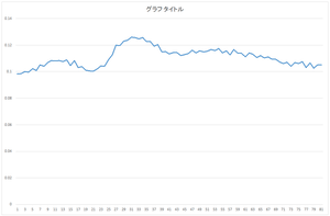
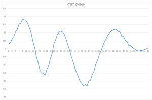
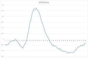
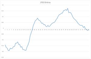
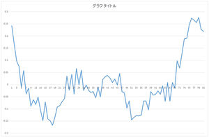
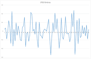
The calculated eigenvector (principal component) (hereafter, orthonormal basis) is ouput to eigenvector.csv file. In this case, the number of bases is 30, and the dimension of bases is 81.

eigenvector.csv


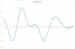0the basis	1st basis	2nd basis	3rd basis
		...
4th basis	5the basis	...	29th basis

Eigenvalue, scree plot, cumulative variance

Calculated eigenvalue is output to eigenvalue.csv file. OpenCV's PCA function sorts the eigenvalues from large to small, and output eigenvalue and eigenvector in this order. Some numerical software library may not sort the eigenvalue, so be careful.

eigenvalue.csv

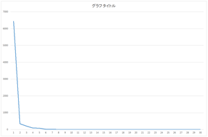
Scree plot

	Eigenvalue	Cumulative variance (%)
0	6436.944	89.6066
1	334.7164	94.266
2	202.1589	97.0802
3	92.20386	98.3638
4	81.9489	99.5046
5	12.75018	99.682
6	8.279398	99.7973
7	7.02354	99.8951
8	1.859	99.921
9	0.81758	99.9323
...	...	...
29	0.024546	100

This webpage does not care about significant digits.

Is it orthonormal basis?

The calculated basis is really an orthonormal basis? Of course, numerical software library correctly calculates orthonormal bases. However, depending on the programmers' bug, such as index is wrong, row and column are swapped, misunderstanding float/double datatype in file input/output, calling the function is wrong, the calculated orthonormal might be wrong due to such human error.

Let's check the basis of 0th and 1st in eigenvector.csv.

0th basis	0.098284	0.098572	...	0.105024
1st basis	0.03047	0.037314	...	0.005358

Let's square the length of 0th basis. Namely, let's calculate the dot product of 0th basis and 0th basis.
0.098284*0.098284 + 0.098572*0.098572 + ... + 0.105024*0.105024 = 1
The result is 1. It is normalized. The length is 1.

Let's calculate the dot product of 0th basis and 1st basis.
0.098284*0.03047 + 0.098572*0.037314 + ... + 0.105024*0.005358 = -4.2E-07
The result is 0. Since the dot product is 0, the 0th basis and the 1st basis is orthogonal in 90 degrees.
By the way, actual result is in the order of 10 to the -7th power, not 0. Due to numerical calculation error, the value does not coincide restrictly to 0. 10 to the -7th power is enough small, and we can think that the calculation is correct.
The above result uses the CSV file. If you use double datatype which is actually calculated, the result will be quite close to 0.
Note that this program output only 6 or 7 digits values to CSV file. We have to use more digits in outputting. More to say, if we need as correct calculation as possible, we should not output ascii-type file, but we should output binary-type file.

We can check whether the output data are orthonormal bases if we calculate for 30-times-30 combination for 30 numbers of bases.

Coefficient, reconstruction, dimension reduction (data in database)

Data can be represented by linear sum of orthonormal bases. Since bases are orthonal with length 1, the coefficient can be calculated from the dot product between data and basis.

I explain one of the data in input.csv.

0th data

7.476484

7.588744

...

6.170647

0th data

I use the basis in eigenvector.csv.

0th basis	0.098284	0.098572	...	0.105024
1th basis	0.03047	0.037314	...	0.005358
...	...	...	...	...
29th basis	0.023033	0.035938	...	0.020174

Let's calculate the dot product between the data and the 0th basis.
7.476484*0.098284 + 7.588744*0.098572 + ... + 6.170647*0.105024 = 57.6941
Next, let's calculate the dot product between the data and the 1st basis. Continue this calculation until 29th basis.

Coefficient 0	57.6941
Coefficient 1	20.21016
...	...
Coefficient 29	0.417814

This data is the sum of the basis 0 multiplied by 57.6941, the basis 1 multiplied by 20.21016, ..., the basis 29 multiplied by 0.417814.

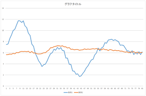
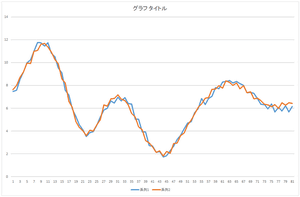
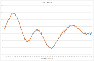
Let's check. Here, orange line represents the reconstructed data. For comparison, the original data is represented by blue line.

First, let's look at the basis 0 multiplied by 57.6941.

=57.6941*

The height is similar but the shape is different.

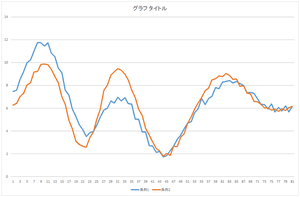
Next, let's add the basis 0 multiplied by 57.6941 and the basis 1 multiplied by 20.21016.

=57.6941*

+20.21016*

Ah! Although not coincide, the position of hill and valley has strong correlation.

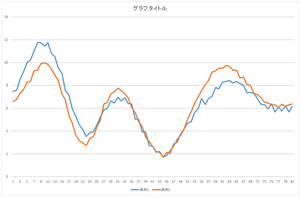
Then, let's add the basis 2 multiplied by -6.59638 to it.

	=57.6941*		+20.21016*
	-6.59638*

Center mountain among 3 mountaines became closer.

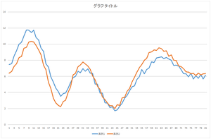
Now, let's add the basis 3 multiplied by -2.05588. And, let's add the basis 4 multiplied by -8.48551. Also, let's add the basis 5 multiplied by -0.81974.


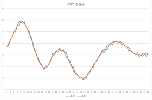Linear sum of 4 bases	Linear sum of 5 bases	Linear sum of 6 bases

Wow! The data can be represented by the linear sum of 5 bases. Almost coinciding. This data can be represented by only 5 values such as 57.6941, 20.21016, ..., -8.48551. Originally, 81 dimension vector is represented by 81 values. Dimension compression (dimension reduction) worked. By the way, we also need the data of 5 bases.

The above characteristics are also same for all data. Namely, 5 bases can be used as common data for all data. Original data was 81 dimension times 30 numbers, namely, 2430 values in total. The data of 5 bases is 81 dimension times 5 numbers, namely, 405 values in total. Each datum have 5 coefficients, so 5 coefficients times 30 numbers, namely, the coefficients are represented by 150 values in total. Original data was 2430 values, but if we represent them using 5 bases, 405+150, namely, 555 values are enough to represent them. The cumulative variance is 99% if we use top 5 bases, thus, the data can be reresented by only 5 bases.

Let's look at 10 bases, 20 bases, and 30 bases.


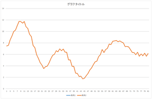Linear sum of 10 bases	Linear sum of 20 bases	Linear sum of 30 bases

The result of all bases coincide with the original data. The conincidence means that the orthonormal bases are correctly calculated. You can your program whether it is working correctly or not.

Coefficient, reconstruction, dimension reduction (data not in database)

Previous section calculated the orthonormal bases using the data included in the databese. How about the data not included in the database? Of course, the data definitely unrelated to the database cannot be represented. The data which has similar characteristics with the database can be somewhat represented.

Let's try. Here, the following data are used. The data which is not the same as either of 30 numbers of data in the database. But this data is artificially made with the same process as the 30 data in the database. Ignore 0th and 1th column, and the data is in 2nd and following columns.

30,data,6.344431462,5.430898881,5.788639826,5.045229125,5.431892473,5.148220769,6.247373877,5.904194559,7.018074794,6.853070842,7.415329243,6.681988468,6.727157704,6.11986334,5.356518341,3.883507699,3.147294817,2.107047233,1.869116159,1.435888089,2.472218576,3.148463328,5.474887965,6.808852152,9.754161136,11.44291821,13.73814761,15.21636521,17.02755852,17.65958085,18.78936127,18.3784868,18.07623842,17.13773537,16.15088152,15.03479419,14.18649566,12.65270032,12.20506825,10.94330218,11.02097082,9.868306121,10.20558999,9.395713825,9.683573142,8.775098307,9.136104211,8.448576259,8.710518542,8.128894893,8.378028257,7.922065916,8.327601559,7.920895667,8.506691436,7.93707303,8.24039303,8.249018074,8.380909421,7.936294965,7.803814733,7.595547706,7.677032829,6.61975181,6.951851616,6.695002513,6.769159695,6.5293568,7.141983556,7.144552264,7.869557545,8.139635591,8.56538665,8.245594894,9.134050718,8.457703754,9.08932824,8.477642682,9.124245036,8.682046072,9.196553879

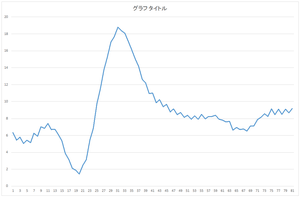
Let's calculate the coefficients as the dot product between this data and 30 bases.

Coefficient 0	79.59188
Coefficient 1	2.800714
...	...
Coefficient 29	-0.11978

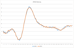
Let's reconstruct using these coefficients.


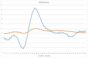Reconstruction using 1 basis	Reconstruction using 2 bases	Reconstruction using 3 bases

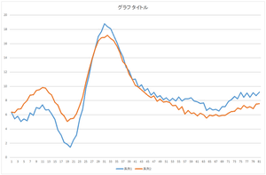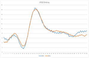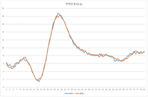Reconstruction using 4 bases	Reconstruction using 5 bases	Reconstruction using 6 bases

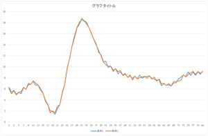Reconstruction using 10 bases	Reconstruction using 20 bases	Reconstruction using 30 bases

The linear sum of 6 bases looks quite similar to the original data. The original data cannot be completely represented even if all 30 bases are used.

Reconstruction of defect data

The groundtruth.csv is artificially generated which is not included in the database.

groundtruth.csv

Suppose that we have a defect data as follows. Suppose that we know the defect position. 0th row of holedata.csv is the data, and 1st row of holedata.csv is the defect position. Here, 1 means the effective data, and 0 means the defect.

holedata.csv

The defect is, for example in computer vision field, outlier such as specular reflection or shadow. Another example is the image to be deleted (for example, suppose that we want to eliminate the texts from TV video).

Let's fill in the defect area. Calculate coefficients of orthonormal basis from defect area. Reconstruct the data using such coefficient.

Let's use top 5 bases, this time, as orthonormal bases. These are included in eigenvector5.csv file.

eigenvector5.csv

Iterative solution

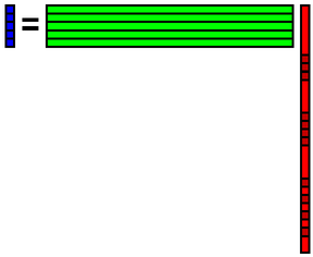
Suppose that we represent the basis as 81 rows 5 columns matrix A, and the coefficient as 5 dimensions column vector x, and the data as 81 dimensions column vector b. The following Ax=b means that the data is represented by linear sum of bases.

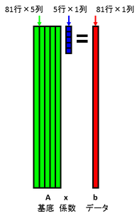
Suppose that the data b is partially defected. Suppose that a certain initial value is embedded in the defect area. Below figure represents the defect as black. Calculate coefficient as the dot product between the data and the bases. This calculation is represented as the matrix calculation x = A⁺ b. Here, A⁺ is a pseudo-inverse of A. A is a concatenation of orthonormal basis, and thus, pseudo-inverse of A becomes transpose of A. Therefore, the coefficient can be calculated as x = A^T b.

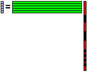
Data b can be reconstructed from the calculated coefficient x and bases A. Namely, we calculate b = A x.

Embed the reconstructed data into the defect area of original data. Again, calculate coefficient x from the data b.

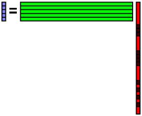
Reconstruct the data b from the coefficient x.

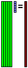
Embed the reconstructed data into the defect area of original data. Again, calculae coefficient x from the data b.

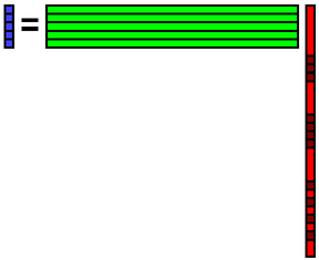
Reconstruct data b from the coefficient x.

Embed the reconstructed data into the defect area of original data. Again, calculate coefficient x from the data b.

Reconstruct data b from the coefficient x.

Interatively calculate as such, the defect data can be repaired. In case the defect area is enough small and the effective pixel is enough large.

This iterative approach is recommended if your algorithm iteratively repairs the defect area.

Direct solution

I explain another approach. First, embed zero into the defect area of both data b and bases A.

Coefficient x can be calculated as x = A⁺ b. A is not orothonormal bases, thus, you cannot use its transpose, but should calculate pseudo-inverse using SVD or so. Set cv::DECOMP_SVD to the 4th argument of OpenCV's cv::solve function, and you will obtain x = A⁺ b.

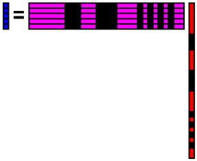
Data b can be reconstructed using the coefficient x and the original bases A.

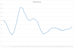
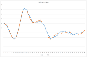
Below shows the program. Calculated coefficient is coefficient.csv, and the reconstructed data is filldata.csv.

coefficient.csv
filldata.csv


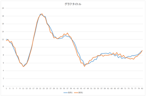Reconstructed data	Reconstructed data (blue) and original defect data (orange)	Reconstructed data (blue) and ground truth (orange)

#include "stdafx.h"

#if _DEBUG
#pragma comment(lib, "opencv_core2411d.lib")
#pragma comment(lib, "opencv_highgui2411d.lib")
#pragma comment(lib, "opencv_imgproc2411d.lib")
#else
#pragma comment(lib, "opencv_core2411.lib")
#pragma comment(lib, "opencv_highgui2411.lib")
#pragma comment(lib, "opencv_imgproc2411.lib")
#endif

#include <opencv2/opencv.hpp>
#include <conio.h>

int main()
{
char filename[256];
FILE* fp;
char line[1024];
int EIGENNUM;
int DIMENSION;
cv::Mat eigenorig;
char* context;
cv::Mat data;
cv::Mat hole;
cv::Mat eigenhole;
cv::Mat coef;

// file open
printf("eigenvector file name = ");
scanf_s("%255s", filename, 256);
if (fopen_s(&fp, filename, "rt")) {
    printf("file open error: %s\n", filename);
    printf("push any key\n");
    _getch();
    return 1;
}

// read header
fgets(line, 1023, fp);
sscanf_s(line, "%d,%d", &EIGENNUM, &DIMENSION);
printf("number of eigenvector = %d\n", EIGENNUM);
printf("number of dimension = %d\n", DIMENSION);

// read data
eigenorig.create(DIMENSION, EIGENNUM, CV_64F);
for (int n = 0; n < EIGENNUM; n++) {
    fgets(line, 1023, fp);
    strtok_s(line, ",", &context);
    strtok_s(NULL, ",", &context);
    for (int d = 0; d < DIMENSION; d++) {
      eigenorig.at<double>(d, n) = atof(strtok_s(NULL, ",", &context));
    }
}
fclose(fp);

// file open
printf("data file name = ");
scanf_s("%255s", filename, 256);
if (fopen_s(&fp, filename, "rt")) {
    printf("file open error: %s\n", filename);
    printf("push any key\n");
    _getch();
    return 1;
}

// read data
data.create(DIMENSION, 1, CV_64F);
fgets(line, 1023, fp);
strtok_s(line, ",", &context);
strtok_s(NULL, ",", &context);
for (int d = 0; d < DIMENSION; d++) {
    data.at<double>(d, 0) = atof(strtok_s(NULL, ",", &context));
}

// read data
hole.create(DIMENSION, 1, CV_32S);
fgets(line, 1023, fp);
strtok_s(line, ",", &context);
strtok_s(NULL, ",", &context);
for (int d = 0; d < DIMENSION; d++) {
    hole.at<int>(d, 0) = atoi(strtok_s(NULL, ",", &context));
}
fclose(fp);

// fill zeros
eigenhole.create(DIMENSION, EIGENNUM, CV_64F);
for (int d = 0; d < DIMENSION; d++) {
    if (hole.at<int>(d, 0) == 0) data.at<double>(d, 0) = 0.0;
    for (int n = 0; n < EIGENNUM; n++) {
      if (hole.at<int>(d, 0) == 0) eigenhole.at<double>(d, n) = 0.0;
      else eigenhole.at<double>(d, n) = eigenorig.at<double>(d, n);
    }
}

// calculate coefficients
coef.create(EIGENNUM, 1, CV_64F);
cv::solve(eigenhole, data, coef, cv::DECOMP_SVD);

// reconstruct data
data = eigenorig * coef;

// write coefficients
fopen_s(&fp, "coefficient.csv", "wt");
fprintf(fp, "%d\n", EIGENNUM);
for (int n = 0; n < EIGENNUM; n++) {
    fprintf(fp, "%d,%lf\n", n, coef.at<double>(n, 0));
}
fclose(fp);

// write reconstructed data
fopen_s(&fp, "filldata.csv", "wt");
fprintf(fp, "1,%d\n", DIMENSION);
fprintf(fp, ",,");
for (int d = 0; d < DIMENSION; d++) {
    fprintf(fp, "%lf", data.at<double>(d, 0));
    if (d < DIMENSION - 1) fprintf(fp, ",");
    else fprintf(fp, "\n");
}
fclose(fp);

// finish
printf("push any key\n");
_getch();
return 0;
}

Back